15 Database Concepts Every Developer Should Know (Explained Simply)
If you've ever written a query that worked but took forever to run, or designed a schema that fell apart under real traffic, you already know: writing SQL and understanding databases are two very different skills.
Most developers learn just enough SQL to get by — SELECT, INSERT, JOIN — but never dig into why databases behave the way they do. That gap is exactly where slow queries, scaling nightmares, and 3 a.m. production incidents come from.
In this post, I'm breaking down 15 core database concepts that separate developers who use databases from developers who understand them. Whether you're prepping for a system design interview, building a high-traffic app, or just want to level up, this guide is for you.
Table of Contents
- Database Indexing
- Database Sharding
- Transactions & ACID
- Normalization (1NF, 2NF, 3NF, BCNF)
- SQL vs NoSQL
- OLTP vs OLAP
- Database Migrations
- MVCC (Multi-Version Concurrency Control)
- Disk vs Memory Access
- Connection Pooling
- Query Optimization
- Database Partitioning
- CAP Theorem
- Optimistic vs Pessimistic Locking
- CQRS (Command Query Responsibility Segregation)
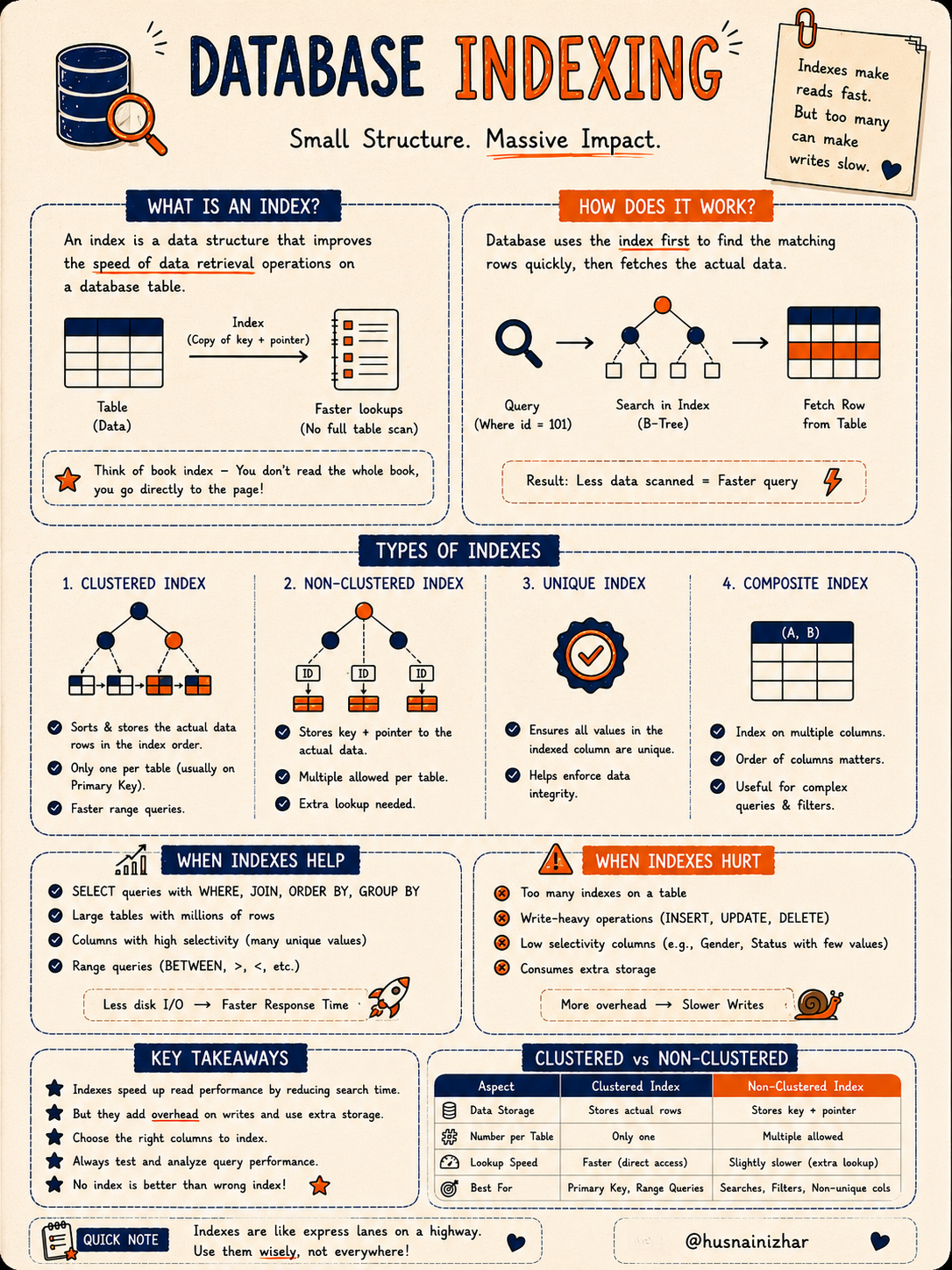
1. Database Indexing
Small structure. Massive impact.
An index is a data structure that speeds up data retrieval on a table — without it, the database has to scan every row to find what you're looking for (a "full table scan").
Think of it like a book index: you don't read the whole book to find a topic, you jump straight to the page. Similarly, when you run a query like WHERE id = 101, the database uses the index (often a B-Tree) to locate the matching row instantly instead of scanning the entire table.
Types of indexes:
- Clustered Index – sorts and stores the actual data rows in index order. Only one per table (usually the primary key). Great for range queries.
- Non-Clustered Index – stores just the key and a pointer to the actual data. You can have multiple per table, but it needs an extra lookup step.
- Unique Index – ensures all values in a column are distinct, enforcing data integrity.
- Composite Index – built on multiple columns; column order matters and it's great for complex filters.
When indexes help: SELECT queries with WHERE, JOIN, ORDER BY, GROUP BY; large tables; high-selectivity columns; range queries.
When indexes hurt: Too many indexes on one table, write-heavy workloads (INSERT/UPDATE/DELETE get slower), low-selectivity columns (like gender or status), and extra storage overhead.
Key takeaway: Indexes trade write performance for read performance. Choose the right columns to index — no index is better than the wrong index.
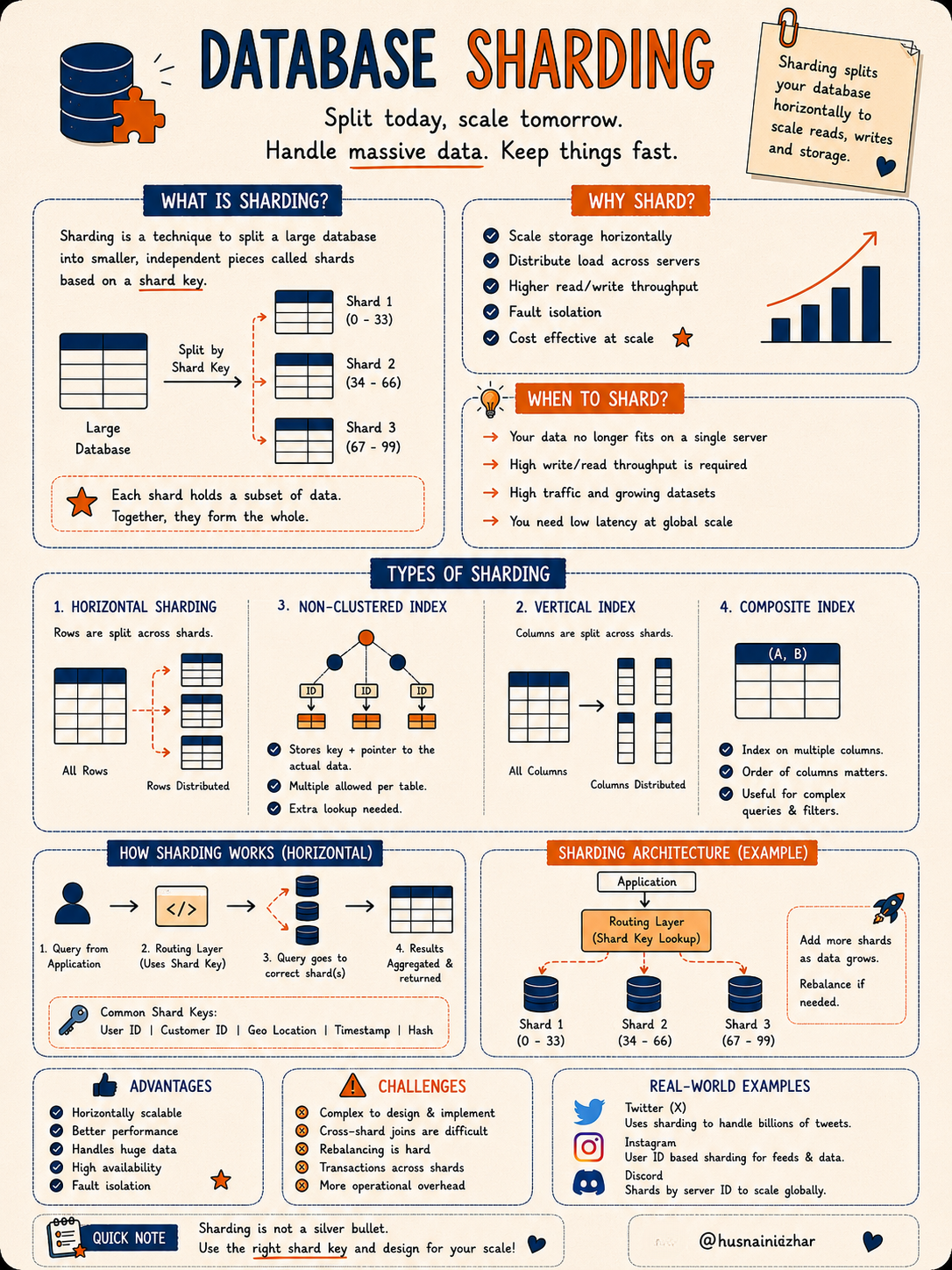
2. Database Sharding
Split today, scale tomorrow.
Sharding is a technique for splitting a large database into smaller, independent pieces called shards, based on a shard key (like User ID, Geo Location, or Timestamp). Each shard holds a subset of the data — together, they form the whole dataset.
Why shard?
- Scale storage horizontally
- Distribute load across servers
- Higher read/write throughput
- Fault isolation
- Cost-effective at scale
How it works: A request comes from the application → a routing layer looks up the shard key → the query is sent to the correct shard(s) → results are aggregated and returned.
Types of sharding:
- Horizontal Sharding – rows are split across shards (most common)
- Vertical Sharding – columns are split across shards
Real-world examples: Twitter (X) shards to handle billions of tweets, Instagram shards by User ID for feeds, and Discord shards by server ID to scale globally.
Challenges: Complex to design, cross-shard joins are difficult, rebalancing is hard, and transactions across shards are tricky.
Key takeaway: Sharding isn't a silver bullet — pick the right shard key and design for your actual scale, not hypothetical scale.
3. Transactions & ACID
All or nothing. No in-between.
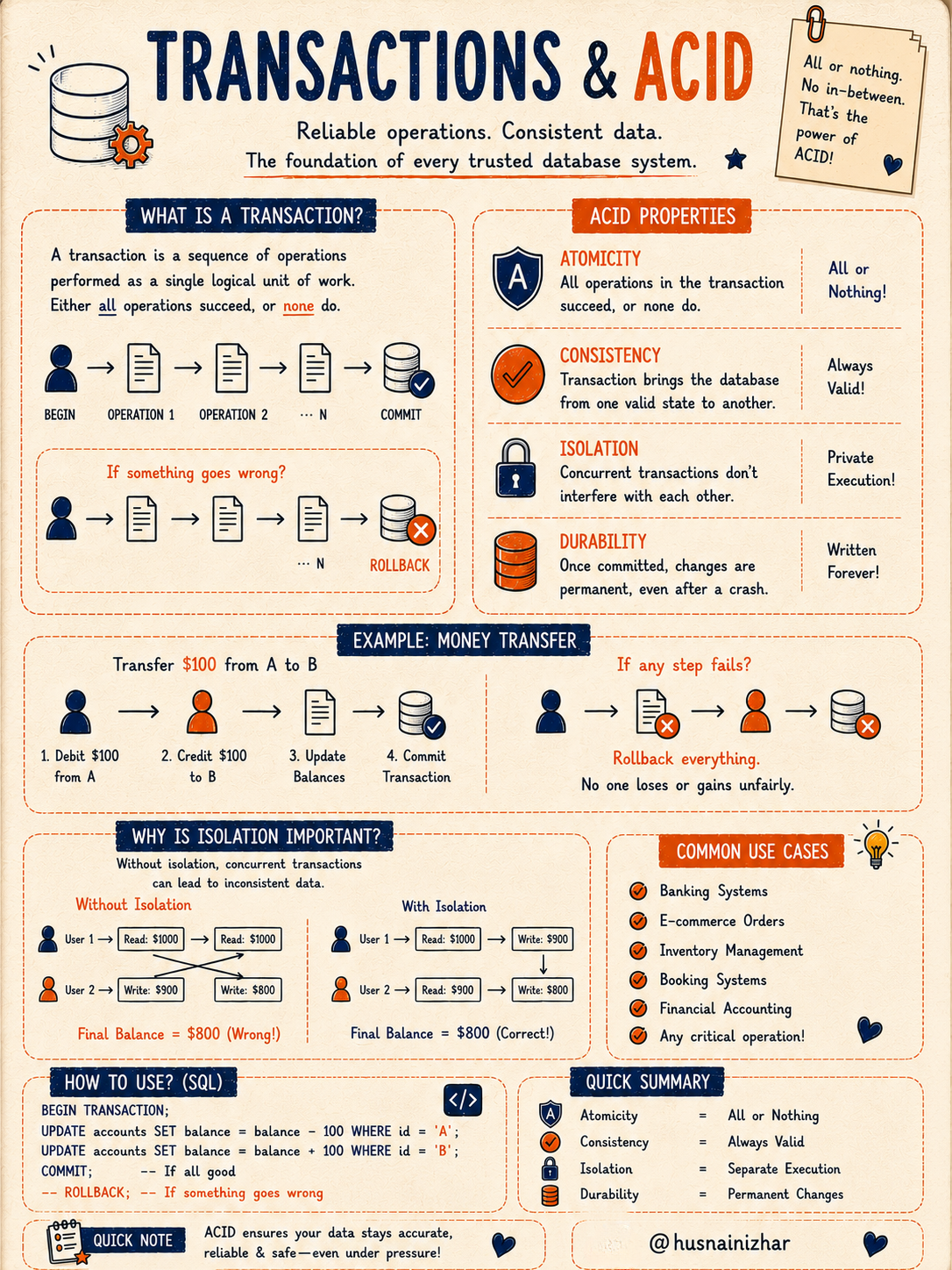
A transaction is a sequence of operations executed as a single logical unit of work — either all operations succeed, or none do. This is the foundation of every trusted database system.
The ACID properties:
- Atomicity – all operations succeed or none do (all or nothing)
- Consistency – the transaction brings the database from one valid state to another
- Isolation – concurrent transactions don't interfere with each other
- Durability – once committed, changes are permanent, even after a crash
Example — money transfer: Debit $100 from Account A → Credit $100 to Account B → Update balances → Commit. If any step fails, everything rolls back. No one loses or gains unfairly.
Why isolation matters: Without it, two concurrent transactions reading and writing the same balance can produce inconsistent results (a classic race condition). With proper isolation, operations happen safely in sequence, avoiding data corruption.
Common use cases: Banking systems, e-commerce orders, inventory management, booking systems, and financial accounting — basically, anywhere correctness can't be compromised.
4. Normalization (1NF, 2NF, 3NF, BCNF)
Good structure today, perfect data tomorrow.
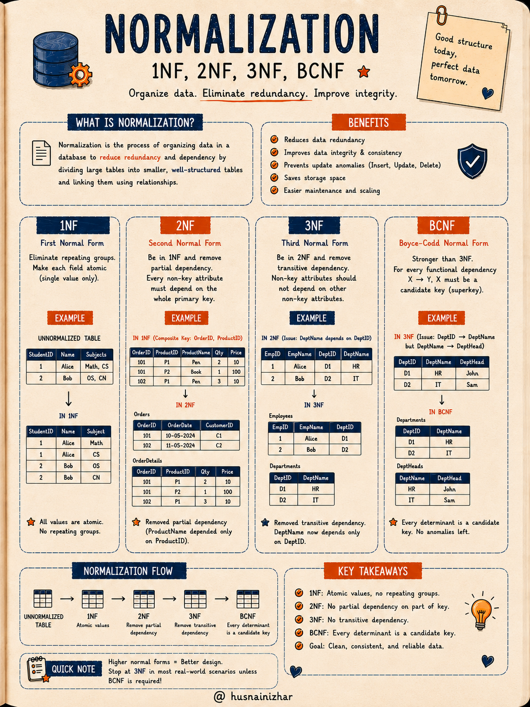
Normalization is the process of organizing data to reduce redundancy and dependency by splitting large tables into smaller, well-structured ones linked by relationships.
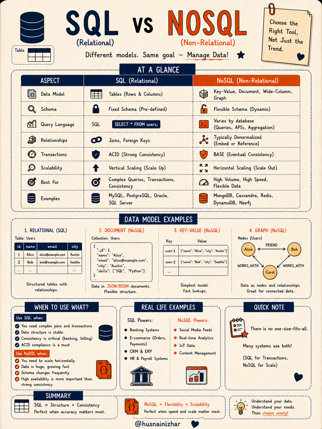
- 1NF (First Normal Form): Eliminate repeating groups — make every field atomic (single-valued).
- 2NF (Second Normal Form): Be in 1NF and remove partial dependency — every non-key attribute must depend on the whole primary key.
- 3NF (Third Normal Form): Be in 2NF and remove transitive dependency — non-key attributes shouldn't depend on other non-key attributes.
- BCNF (Boyce-Codd Normal Form): Stronger than 3NF — for every functional dependency X → Y, X must be a candidate key (superkey).
Benefits: Reduces redundancy, improves data integrity, prevents update anomalies, saves storage, and makes maintenance/scaling easier.
Practical tip: In most real-world systems, stopping at 3NF is enough. Push to BCNF only when strictly required — over-normalizing can hurt query performance by requiring more joins.
5. SQL vs NoSQL
Different models. Same goal — manage data.
| Aspect | SQL (Relational) | NoSQL (Non-Relational) |
|---|---|---|
| Data Model | Tables (rows & columns) | Key-Value, Document, Wide-Column, Graph |
| Schema | Fixed, pre-defined | Flexible, dynamic |
| Relationships | Joins, foreign keys | Denormalized (embed or reference) |
| Transactions | ACID (strong consistency) | BASE (eventual consistency) |
| Scalability | Vertical (scale up) | Horizontal (scale out) |
| Examples | MySQL, PostgreSQL, Oracle | MongoDB, Cassandra, Redis, DynamoDB |
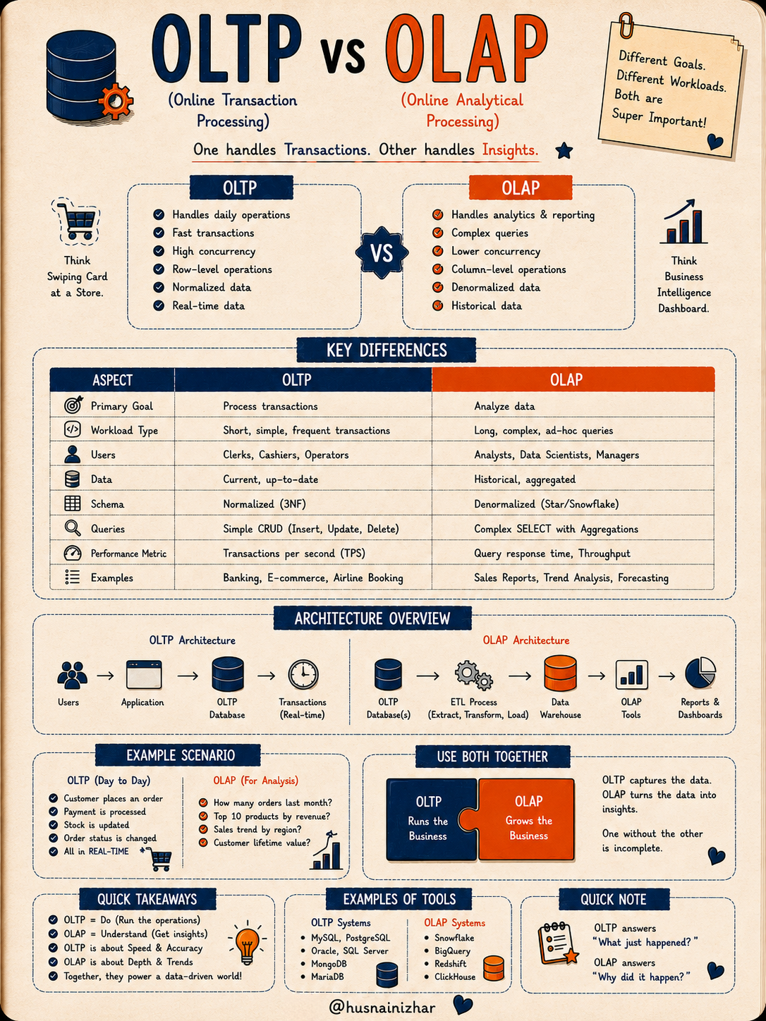
Use SQL when: you need complex joins and transactions, your data structure is stable, and ACID compliance is a must (banking, ERP, CRM).
Use NoSQL when: you need to scale horizontally, data is huge and growing fast, schema changes frequently, and availability matters more than strict consistency (social feeds, IoT data, real-time analytics).
Key takeaway: There's no one-size-fits-all. Many modern systems use both — SQL for transactions, NoSQL for scale.
6. OLTP vs OLAP
One handles transactions. The other handles insights.
OLTP (Online Transaction Processing): Handles daily operations — fast transactions, high concurrency, row-level operations, normalized real-time data. Think: swiping a card at a store. Examples: banking, e-commerce, airline booking.
OLAP (Online Analytical Processing): Handles analytics and reporting — complex queries, column-level operations, denormalized historical data. Think: a business intelligence dashboard. Examples: sales reports, trend analysis, forecasting.
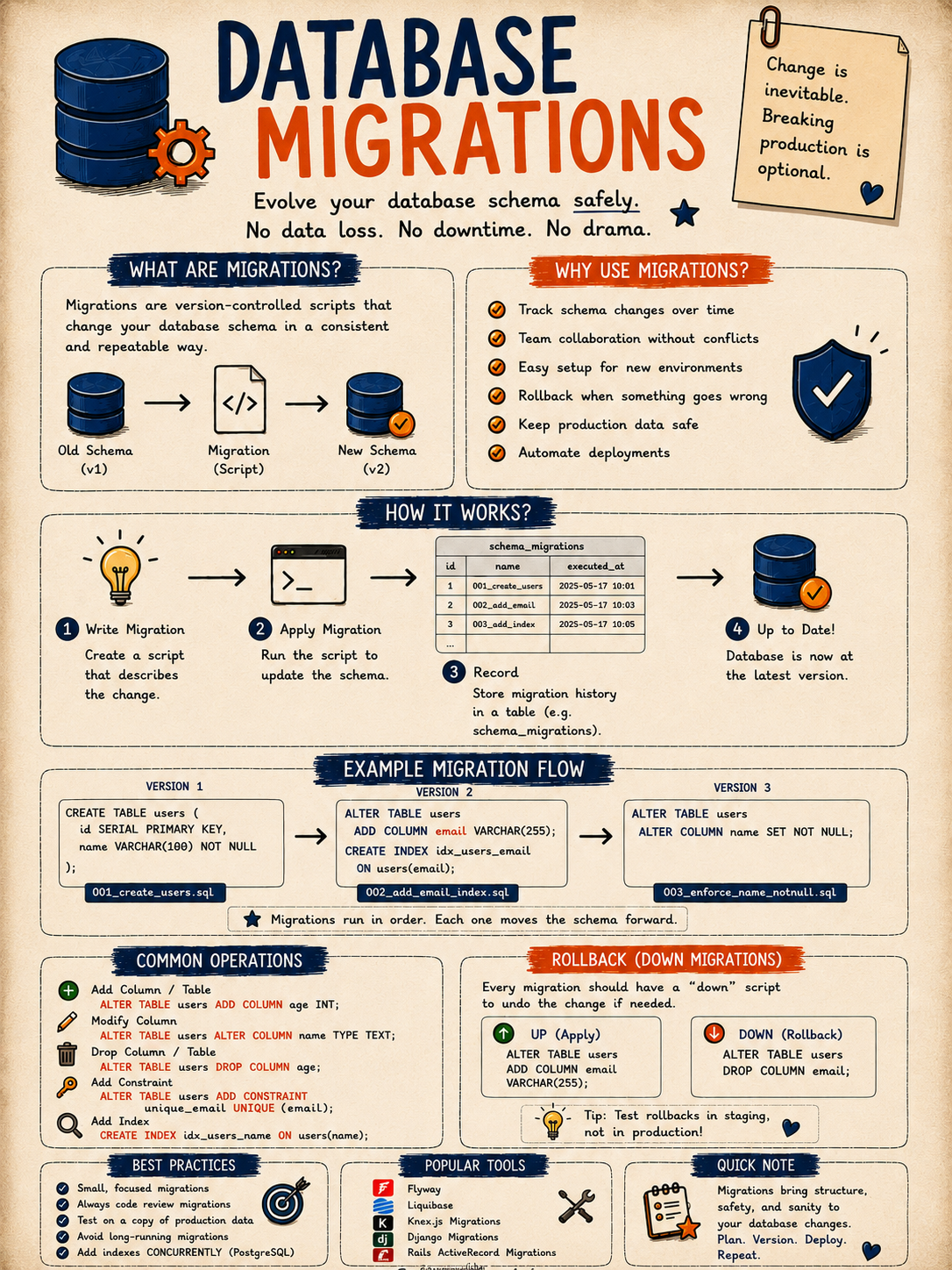
Architecture overview: OLTP data flows through an ETL process (Extract, Transform, Load) into a data warehouse, where OLAP tools generate reports and dashboards.
Use both together: OLTP runs the business (captures the data), OLAP grows the business (turns data into insights). One without the other is incomplete.
Simple way to remember: OLTP answers "What just happened?" OLAP answers "Why did it happen?"
7. Database Migrations
Change is inevitable. Breaking production is optional.
Migrations are version-controlled scripts that change your database schema in a consistent, repeatable way — think of them as Git commits for your database structure.
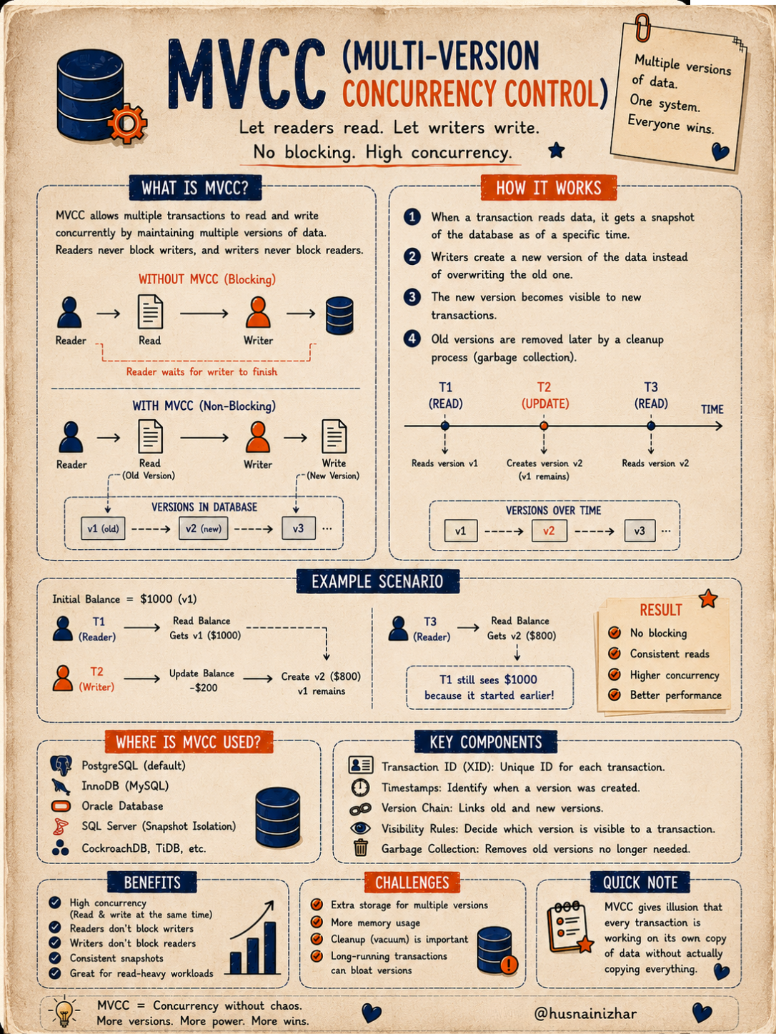
Why use migrations? Track schema changes over time, enable team collaboration without conflicts, easy setup for new environments, rollback capability, and safer, automated deployments.
How it works: Write a migration script → apply it to update the schema → record it in a migration history table (e.g., schema_migrations) → the database is now up to date.
Best practices:
- Keep migrations small and focused
- Always code-review migrations
- Test on a copy of production data
- Avoid long-running migrations
- Add indexes concurrently (especially in PostgreSQL, to avoid locking tables)
- Always write a "down" migration to roll back changes if needed
Popular tools: Flyway, Liquibase, Knex.js Migrations, Django Migrations, Rails ActiveRecord Migrations.
8. MVCC (Multi-Version Concurrency Control)
Let readers read. Let writers write. No blocking.
MVCC allows multiple transactions to read and write concurrently by maintaining multiple versions of data. Readers never block writers, and writers never block readers.
How it works:
- When a transaction reads data, it gets a snapshot as of a specific point in time.
- Writers create a new version of the data instead of overwriting the old one.
- The new version becomes visible to new transactions.
- Old versions are eventually cleaned up (garbage collection/vacuum).
Example: If Transaction 1 reads a balance of $1000 before Transaction 2 updates it to $800, Transaction 1 will still see $1000 — because it started before the update. This gives consistent reads without blocking.
Where it's used: PostgreSQL (default), InnoDB (MySQL), Oracle Database, SQL Server (Snapshot Isolation), CockroachDB, TiDB.
Trade-off: Extra storage for multiple versions, more memory usage, and the need for regular cleanup (vacuuming) — but in exchange, you get much higher concurrency.
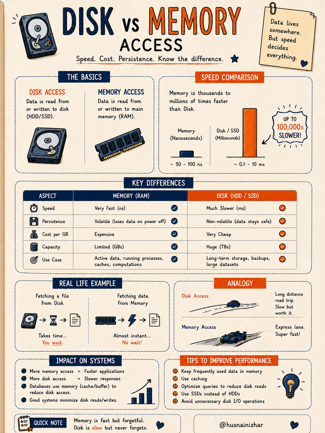
9. Disk vs Memory Access
Data lives somewhere. But speed decides everything.
Disk access: Reading/writing to HDD or SSD — slower (0.1–10 ms), but non-volatile (data survives power loss) and cheap per GB, with huge capacity.
Memory access: Reading/writing to RAM — extremely fast (50–100 nanoseconds), but volatile (data is lost on power off) and expensive per GB, with limited capacity.
Memory is thousands to millions of times faster than disk — up to 100,000x in some cases.
Analogy: Disk access is a long road trip — slow, but reliable. Memory access is the express lane — almost instant.
Impact on systems: Databases use memory (via caching and buffers) to minimize disk access, since more memory access means faster applications, while more disk access means slower responses.
Tips to improve performance: Keep frequently used data in memory, use caching layers, optimize queries to reduce unnecessary disk reads, and prefer SSDs over HDDs where possible.
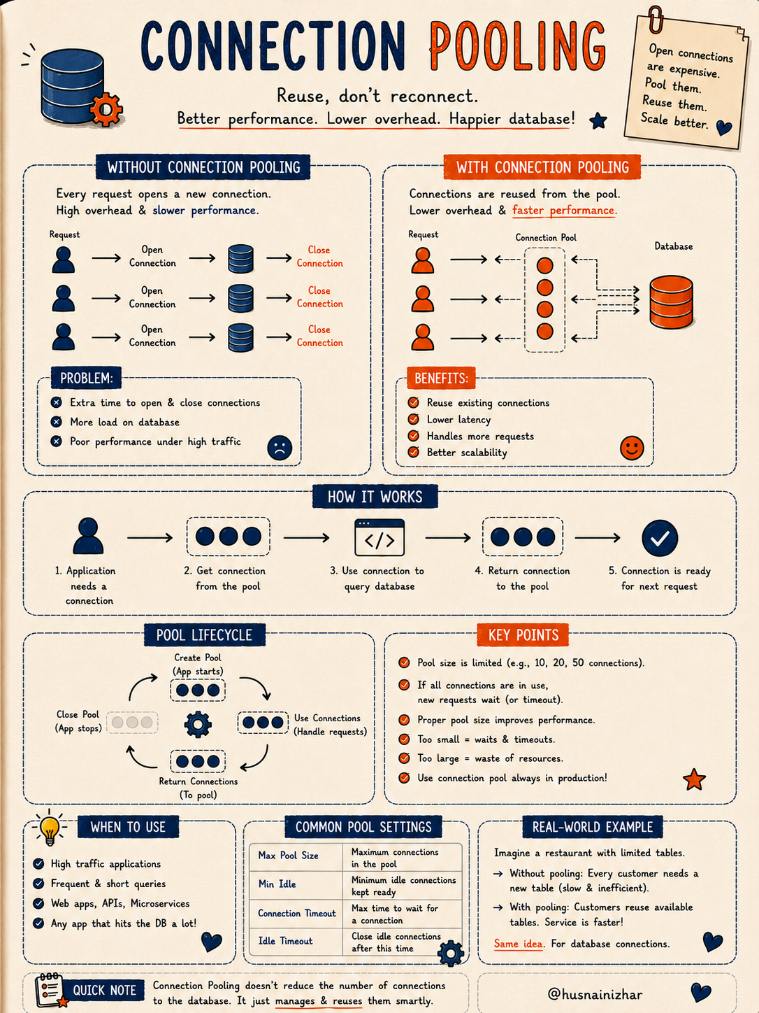
10. Connection Pooling
Reuse, don't reconnect.
Without connection pooling, every request opens a brand-new database connection and closes it afterward — this adds overhead, increases load on the database, and hurts performance under high traffic.
With connection pooling, a pool of pre-established connections is reused across requests instead of constantly opening and closing new ones.
How it works:
- The application needs a connection
- It grabs one from the pool
- Uses it to query the database
- Returns the connection to the pool
- The connection is ready for the next request
Common pool settings:
- Max Pool Size: Maximum number of connections allowed
- Min Idle: Minimum idle connections kept ready
- Connection Timeout: How long to wait for a connection before failing
- Idle Timeout: When to close unused idle connections
Analogy: Think of a restaurant with limited tables. Without pooling, every customer needs a brand-new table built from scratch. With pooling, customers simply reuse available tables — much faster service.
Key takeaway: Connection pooling doesn't reduce the number of connections to the database — it manages and reuses them smartly. Use it in every production application that hits a database frequently.
11. Query Optimization
A slow query is like a tiny leak — at scale, it becomes a big problem.
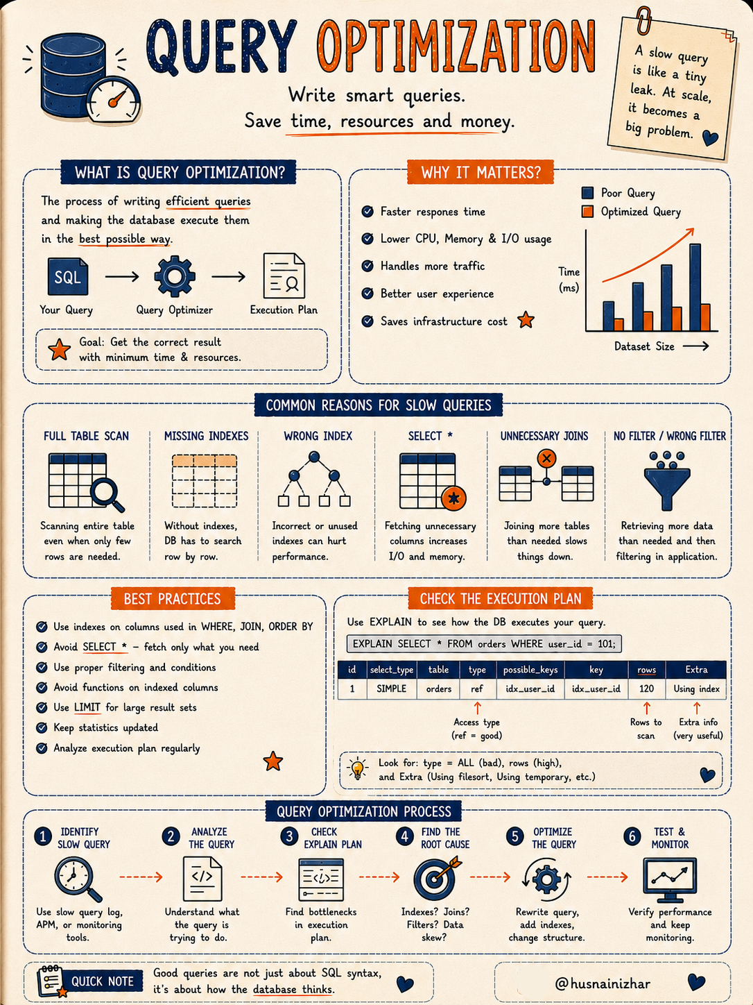
Query optimization is the process of writing efficient queries and helping the database execute them in the best possible way, with the goal of getting correct results using minimum time and resources.
Common reasons for slow queries:
- Full table scans (scanning the entire table when only a few rows are needed)
- Missing indexes
- Using the wrong index
- SELECT * (fetching unnecessary columns)
- Unnecessary joins
- Poor or missing filters
Best practices:
- Use indexes on columns in WHERE, JOIN, and ORDER BY clauses
- Avoid SELECT * — fetch only what you need
- Avoid using functions on indexed columns (it prevents index usage)
- Use LIMIT for large result sets
- Keep table statistics updated
- Regularly analyze execution plans
Checking the execution plan: Use EXPLAIN before your query (e.g., EXPLAIN SELECT * FROM orders WHERE user_id = 101;) to see exactly how the database plans to execute it — look out for type = ALL (a full scan, which is bad) and high row counts.
Optimization process: Identify the slow query → analyze it → check the execution plan → find the root cause → optimize the query → test and monitor the results.
12. Database Partitioning
Split big tables into smaller pieces to boost performance.
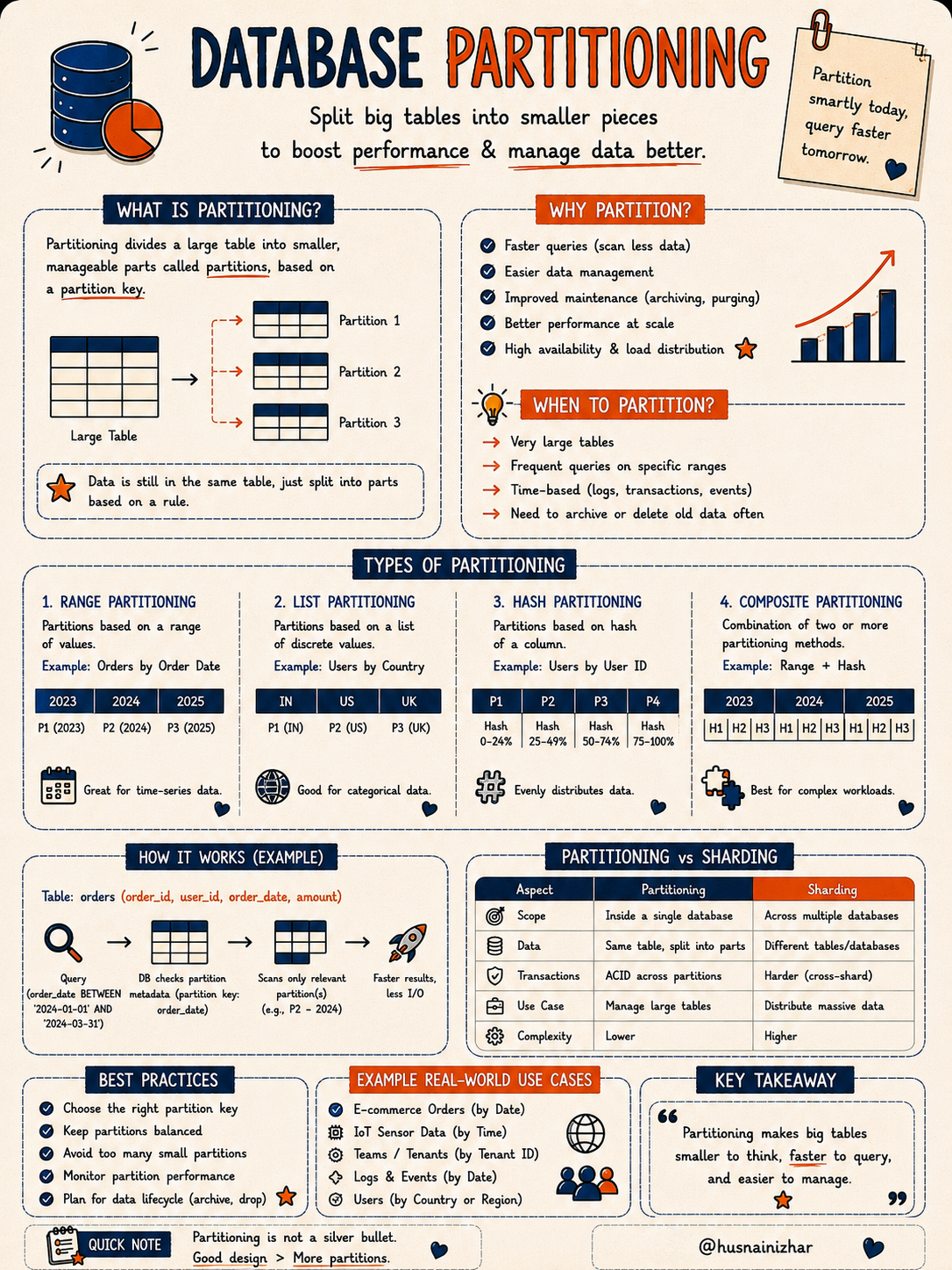
Partitioning divides a large table into smaller, manageable parts called partitions, based on a partition key — the data stays in the same table, just split internally based on a rule.
Types of partitioning:
- Range Partitioning – based on a range of values (e.g., orders by year)
- List Partitioning – based on a list of discrete values (e.g., users by country)
- Hash Partitioning – based on a hash of a column, evenly distributing data
- Composite Partitioning – a combination of two or more methods (e.g., range + hash), best for complex workloads
Partitioning vs Sharding — what's the difference?
| Aspect | Partitioning | Sharding |
|---|---|---|
| Scope | Inside a single database | Across multiple databases |
| Data | Same table, split into parts | Different tables/databases |
| Transactions | ACID across partitions | Harder (cross-shard) |
| Complexity | Lower | Higher |
When to partition: Very large tables, frequent queries on specific ranges, time-based data (logs, transactions, events), or when you need to archive/delete old data often.
Key takeaway: Partitioning makes big tables smaller to think about, faster to query, and easier to manage — but good design matters more than simply adding more partitions.
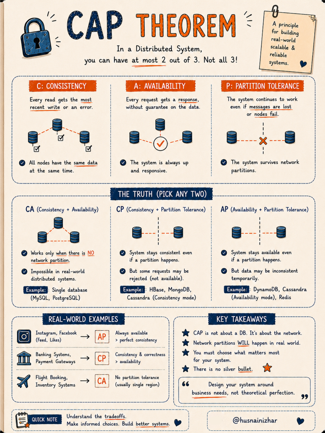
13. CAP Theorem
In a distributed system, you can have at most 2 out of 3. Not all 3.
CAP Theorem states that a distributed system can only guarantee two of the following three properties at the same time:
- Consistency (C): Every read gets the most recent write, or an error.
- Availability (A): Every request gets a response, without a guarantee it's the most recent data.
- Partition Tolerance (P): The system keeps working even if messages are lost or nodes fail.
The three combinations:
- CA (Consistency + Availability): Only works when there's no network partition — essentially impossible in real-world distributed systems. Example: a single database instance (MySQL, PostgreSQL).
- CP (Consistency + Partition Tolerance): Stays consistent during a partition, but some requests may be rejected. Examples: HBase, MongoDB, Cassandra (in consistency mode).
- AP (Availability + Partition Tolerance): Stays available during a partition, but data may be temporarily inconsistent. Examples: DynamoDB, Cassandra (availability mode), Redis.
Real-world examples:
- Instagram/Facebook feeds → AP (availability matters more than perfect consistency)
- Banking systems, payment gateways → CP (correctness matters more than availability)
- Flight booking, inventory systems → CA (usually single-region, no partition tolerance needed)
Key takeaway: Network partitions will happen in the real world. There's no silver bullet — design your system around your actual business needs, not theoretical perfection.
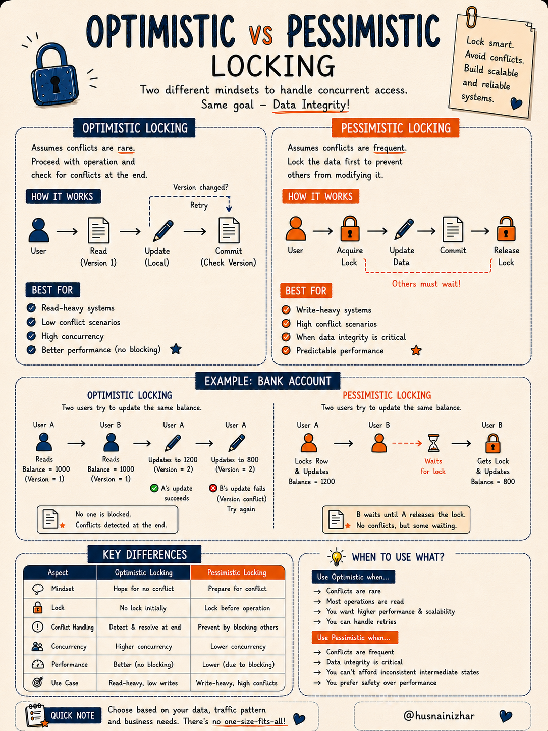
14. Optimistic vs Pessimistic Locking
Two different mindsets to handle concurrent access. Same goal — data integrity.
Optimistic Locking: Assumes conflicts are rare. The system proceeds with the operation and checks for conflicts only at commit time (often via version numbers). If a conflict is found, the operation retries.
Pessimistic Locking: Assumes conflicts are frequent. The system locks the data before the operation begins, forcing other users to wait until the lock is released.
Example — bank account update:
Optimistic: Two users read the same balance (version 1). User A updates first and succeeds. User B's update fails due to a version conflict and must retry.
Pessimistic: User A locks the row and updates it. User B must wait until A releases the lock before making their own update.
When to use optimistic locking: Conflicts are rare, most operations are reads, you want higher performance and scalability, and you can handle retries. Best for read-heavy systems.
When to use pessimistic locking: Conflicts are frequent, data integrity is critical, you can't afford inconsistent intermediate states, and you prefer safety over raw performance. Best for write-heavy, high-conflict systems.
Key takeaway: Choose based on your data patterns and business needs — there's no one-size-fits-all.
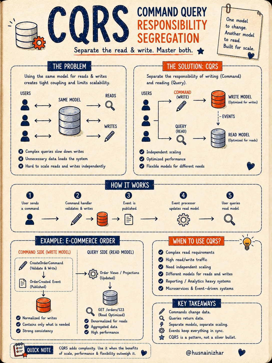
15. CQRS (Command Query Responsibility Segregation)
One model to change. Another model to read. Built for scale.
The problem: Using the same data model for both reads and writes creates tight coupling — complex queries slow down writes, and it becomes hard to scale reads and writes independently.
The solution: CQRS separates the responsibility of writing (Command) from reading (Query) into two distinct models:
- Write Model – optimized for writes, normalized, strongly consistent
- Read Model – optimized for reads, denormalized, aggregated for performance
How it works:
- User sends a command
- The command handler validates and writes the data
- An event is published
- An event processor updates the read model
- The user queries the (separately optimized) read model
Example — e-commerce order: A CreateOrderCommand writes to the normalized write model and publishes an OrderCreated event. That event updates a denormalized "Order Views" projection, which powers a fast GET /orders/123 read endpoint.
When to use CQRS: Complex read requirements, high read/write traffic, need for independent scaling, reporting/analytics-heavy systems, and event-driven microservices.
Key takeaway: CQRS adds real complexity — use it only when the benefits of scale, performance, and flexibility outweigh that cost. It's a pattern, not a silver bullet.
Final Thoughts
Databases are the backbone of almost every application we build — yet most of us only scratch the surface of how they actually work. Understanding these 15 concepts won't just help you pass a system design interview; it'll change how you design schemas, write queries, and debug performance issues in production.

Quick recap:
- Indexing, Partitioning, Sharding → speed and scale
- ACID, Normalization, MVCC → correctness and consistency
- SQL vs NoSQL, OLTP vs OLAP → choosing the right tool for the job
- CAP Theorem, Locking strategies, CQRS → tackling distributed systems trade-offs
- Migrations, Connection Pooling, Query Optimization, Disk vs Memory → the operational backbone that keeps it all running smoothly
There's no single "correct" database setup — only the right trade-offs for your specific use case. Understand the fundamentals, and the right decisions become a lot easier to make.
If you found this useful, follow me for more deep dives into system design and backend engineering — one concept at a time.